A storm hydrograph shows how flow changes, but its peak alone cannot tell you how much water passed the outlet. Paired rainfall and discharge graphs let you practice the missing steps: account for duration, separate a specified baseline, and convert volume to an equivalent depth.
Calculate storm-hydrograph runoff volume by subtracting an assumed baseflow from discharge and integrating the remaining rate over time. Divide that volume by contributing area for equivalent depth. This fictional example gives about 2.29 million cubic feet (64,800 m³), or 0.71 inches (18 mm), under its stated baseline and straight-line assumptions.
1. Read the Supplied Storm Data
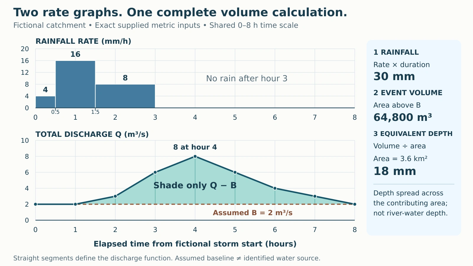
A discharge hydrograph plots water volume per unit time. A hyetograph plots rainfall intensity, meaning depth per unit time. Minnesota DNR distinguishes these graphs; their vertical axes cannot share one physical scale.
Use one imaginary outlet with a supplied contributing area of about 1.39 square miles (3.6 km²). Rainfall is already averaged across that area. Assume no reservoir-operation or snowmelt pulse; the exercise does not infer these conditions from the curve. The river and drainage-basin primer explains the area draining to an outlet.
The graph, tables and arithmetic retain the exact metric inputs so rounded U.S. conversions do not change the answer. Rainfall rates are constant within each listed interval. Straight lines connect consecutive discharge samples, and zero rainfall is specified from hour 3 through hour 8.

2. Multiply Rainfall Rate by Duration
Each rainfall bar contributes rate × duration. Its height alone is not a rainfall amount. The middle bar lasts twice as long as the first, while the third lasts three times as long.
| Elapsed interval (h) | Duration (h) | Rate (mm/h) | Depth (mm) |
|---|---|---|---|
| 0–0.5 | 0.5 | 4 | 2 |
| 0.5–1.5 | 1 | 16 | 16 |
| 1.5–3 | 1.5 | 8 | 12 |
| 3–8 | 5 | 0 | 0 |
Rainfall depth = (4 × 0.5) + (16 × 1) + (8 × 1.5) = 30 mm.
The storm supplies about 1.18 inches (30 mm) of gross rainfall. Over the three rainy hours, its mean rate is about 0.39 inches per hour (10 mm/h). The highest interval rate is about 0.63 inches per hour (16 mm/h), maintained throughout hours 0.5–1.5.
Adding 4 + 16 + 8 produces a sum of rates, not the storm depth. TxDOT’s Hydrograph Method explains the depth-duration relationship; here, multiplying each rate by its own duration preserves the unequal intervals.
3. Subtract the Baseline and Add Trapezoids
Separate the specified event-flow component
Assume a constant baseline B of about 71 cubic feet per second (2 m³/s) throughout hours 0–8. Subtract B from total discharge Q at every sample. This is a supplied separation assumption, not a groundwater contribution uniquely observed in the graph.
| Time (h) | Total Q (m³/s) | Assumed B (m³/s) | Q − B (m³/s) |
|---|---|---|---|
| 0 | 2 | 2 | 0 |
| 1 | 2 | 2 | 0 |
| 2 | 3 | 2 | 1 |
| 3 | 6 | 2 | 4 |
| 4 | 8 | 2 | 6 |
| 5 | 6 | 2 | 4 |
| 6 | 4 | 2 | 2 |
| 7 | 3 | 2 | 1 |
| 8 | 2 | 2 | 0 |
Total discharge peaks at about 283 cubic feet per second (8 m³/s) at hour 4. The flow above the baseline is then about 212 cubic feet per second (6 m³/s). Neither peak is a volume.
Turn each rate-time trapezoid into volume
For each interval, average its two endpoint excess rates, then multiply by elapsed seconds. The hourly intervals each contain 3,600 seconds. For hours 2–3:
Volume = ((1 + 4) ÷ 2) m³/s × 3,600 s = 9,000 m³.
| Interval (h) | Mean Q − B (m³/s) | Volume (m³) |
|---|---|---|
| 0–1 | 0 | 0 |
| 1–2 | 0.5 | 1,800 |
| 2–3 | 2.5 | 9,000 |
| 3–4 | 5 | 18,000 |
| 4–5 | 5 | 18,000 |
| 5–6 | 3 | 10,800 |
| 6–7 | 1.5 | 5,400 |
| 7–8 | 0.5 | 1,800 |
Sum = 0 + 1,800 + 9,000 + 18,000 + 18,000 + 10,800 + 5,400 + 1,800 = 64,800 m³. That is about 2.29 million cubic feet.
The units cancel as (m³/s) × s = m³. Multiplying by hours without conversion gives the wrong volume. Integrating river stage instead would not produce a water volume.
These trapezoids are exact for the supplied straight-line function. With sparse real observations, that interpolation would be an approximation. The window contains the full specified pulse, with zero excess at both endpoints; its exact return to baseline is a teaching idealization.
4. Divide Volume by Contributing Area
Convert the supplied area before dividing: 3.6 km² = 3,600,000 m². Then:
Equivalent depth = 64,800 m³ ÷ 3,600,000 m² = 0.018 m = 18 mm.
The result is about 0.71 inches (18 mm) spread uniformly across the contributing area. Boise State’s Watershed Water Balance explains this volume-to-area conversion. It describes an equivalent layer, not actual river depth, floodwater depth or water covering every part of the land.
Keep the separation assumption attached to the answer
Boise State’s Hydrograph Separation distinguishes event-flow separation from identifying new and old water. The shaded component need not consist entirely of new storm rain or water that traveled over the ground. Another defensible baseline could give another estimated event volume.
The difference from rainfall, about 0.47 inches (12 mm), cannot all be assigned to infiltration, recharge, evaporation or storage. Those claims require additional water-balance information. The water-cycle explanation separates these pathways and stores.
As an error check, integrating all discharge gives about 4.32 million cubic feet (122,400 m³), including 2.03 million cubic feet (57,600 m³) of baseline flow. That is the wrong component. Its equivalent depth of about 1.34 inches (34 mm) exceeding 1.18 inches (30 mm) rainfall is not itself a conservation violation: streamflow can include previously stored water.
Name the rainfall basis before reporting lag
HEC-HMS defines basin lag using the center of mass of excess rainfall. Only gross rainfall is supplied here, so that lag cannot be calculated. The highest rainfall bar also represents an interval, not one unique peak timestamp. For further practice with explicitly stated conventions, try the Hydrology Quiz.
What Did We Learn Today?
Read both axes and preserve interval duration. Subtract the stated baseline before integrating, convert hours to seconds, and divide volume by the matching contributing area. The arithmetic is reproducible; identifying the water’s source or destination requires evidence beyond these graphs.
Sources & Data Notes
All storm values and the diagram are original fictional teaching inputs, not station observations or a forecast. Metric calculations are exact within the stated model; U.S. equivalents are rounded. Sources support terminology and method, not these invented values. The Boise State water-balance exercise uses an annual window; the same dimensional conversion is applied here to the specified event.