Two wells have water 20 feet (6.10 meters) below one measuring point and 12 feet (3.66 meters) below the other. You cannot tell which has the higher groundwater level from those depths alone. First, you need to know the elevations of the measuring points and whether the wells observe comparable groundwater conditions.
To compare groundwater levels, subtract each well’s depth to water from the elevation of the exact measuring point, using the same datum. Then check that the wells observe comparable aquifer conditions. A water table describes an unconfined system; a confined well’s level can reflect pressure rather than the top of saturated material.
How to use this article: You can separate storage from flow, interpret a confined well, compare two water-level readings, or understand changing well levels.
Compare Water-Level Elevations, Not Just Depths
Use the same datum and the correct measuring point
Hydraulic head describes groundwater’s hydraulic potential as a water-level elevation relative to a datum, the shared elevation reference. For a nonflowing observation well, calculate water-level elevation by subtracting depth to water from the elevation of the point used to measure that depth. Victoria’s water-monitoring guidance explains this calculation and the need to account for offsets between measuring points.
Consider two fictional wells observed simultaneously in the same connected unconfined aquifer. Both have suitable shallow screened intervals, equilibrated levels, negligible vertical gradients and no recent pumping disturbance. Their measuring points were surveyed against the same local datum.
| Well | Measuring-point elevation | Depth below that point | Water-level elevation |
|---|---|---|---|
| A | 150 ft (45.72 m) | 20 ft (6.10 m) | 130 ft (39.62 m) |
| B | 135 ft (41.15 m) | 12 ft (3.66 m) | 123 ft (37.49 m) |
Well A has the deeper depth-to-water reading, yet its water-level elevation is 7 feet (2.13 meters) higher. The calculation is 150 − 20 = 130 feet for A and 135 − 12 = 123 feet for B.
These two readings establish a head difference between the locations, not a complete two-dimensional flow map or a groundwater speed. More observations and geological information are needed to interpret the wider pattern. Do not assume a parcel of water travels directly from one well to the other.
The Groundwater Project’s head-mapping explanation describes common-datum measurements, screened intervals and measurement uncertainty. A measuring point at the top of a casing is not automatically the same elevation as the ground beside it.
An Aquifer Is Water-Bearing Material, Not Usually a Cavern
Porosity and permeability answer different questions
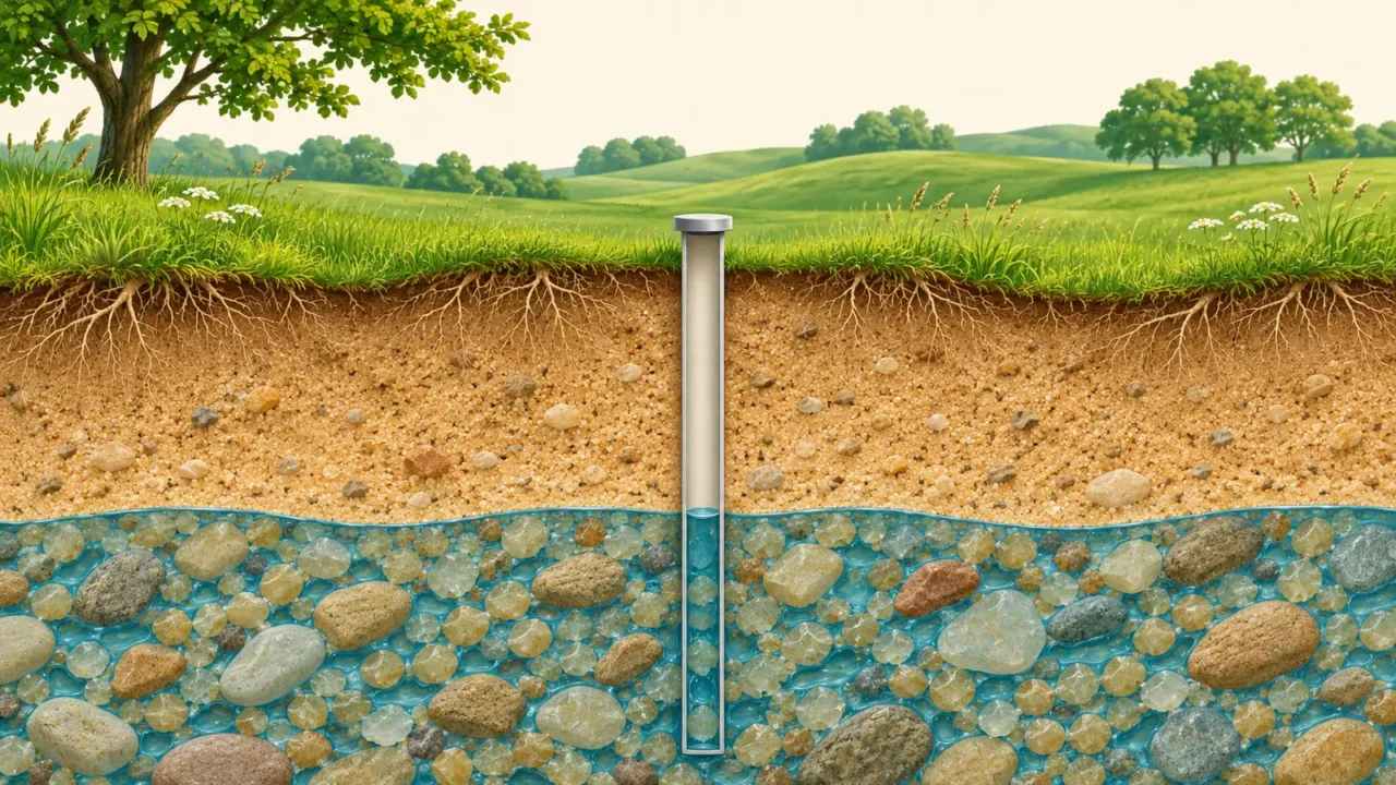
Most groundwater occupies pores between grains or fractures in rock. An aquifer is the formation that can transmit useful quantities of that water to a well or spring. A saturated material that releases water only very slowly is not automatically a useful aquifer.
USGS distinguishes water storage from transmission. Porosity describes how much of a material’s volume is open space. Permeability describes how readily fluid can pass through it. The size and connections of pores and fractures matter, not just their combined volume.
Sand, gravel, sandstone and fractured rock can form aquifers under suitable conditions. Some limestone systems contain large solution channels, but the image of every aquifer as an underground lake is misleading.
The British Geological Survey glossary also distinguishes permeability, a property of the material, from hydraulic conductivity, which accounts for the fluid as well. These concepts help explain why equal-looking stores need not supply wells at equal rates.
The Water Table Belongs to an Unconfined System
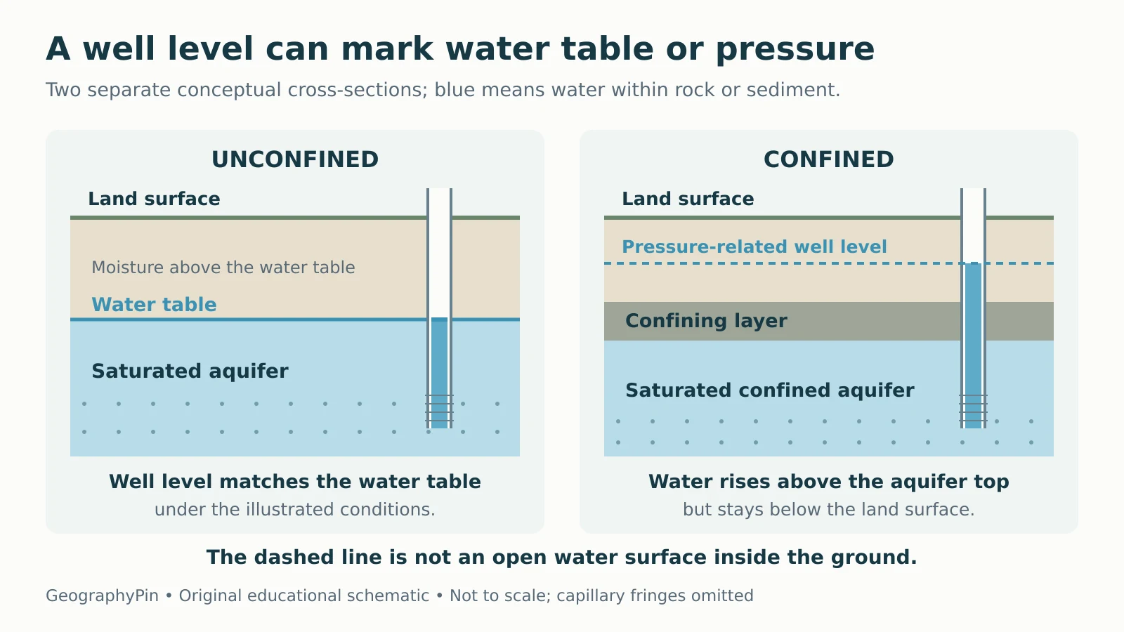
In an unconfined groundwater system, the water table is the surface where groundwater pressure equals atmospheric pressure. It is commonly described as the upper surface of the saturated zone. It can rise and fall as conditions change.
Material above it is not necessarily dry. The unsaturated zone can contain moisture, and capillary forces can draw water above the water table. A simple diagram often omits that capillary fringe, so its color boundary is a teaching simplification.
Water entering the soil is not automatically groundwater recharge. Some remains near the surface or returns to the air through evaporation and plant use. The water-cycle guide explains those pathways.
A well’s design matters. A shallow observation well connected to the appropriate part of an unconfined aquifer can show its water level. A deep well open to several formations can mix their pressure signals instead. BGS’s level terminology explains why the monitored interval must be known.
A Confined Well Can Show a Pressure Level
Artesian does not always mean overflowing
A confined aquifer is saturated beneath a relatively low-permeability confining layer. Water can be under enough pressure to rise in a properly cased well above the top of the aquifer. That level is not an underground air-water boundary at the same height.
The imaginary surface traced by these well levels is a potentiometric surface. In broader technical usage, a water table is also a kind of potentiometric surface; naming the aquifer and conditions avoids confusion.

As USGS explains artesian wells, water may rise above a confined aquifer without reaching the ground surface. It is a flowing artesian well only when pressure is sufficient for water to flow out without pumping. A deep well is not automatically artesian.
For example, a confined aquifer’s top might lie well below a static well level that still remains below the well outlet. That is consistent with confinement and pressure; the absence of a fountain does not prove the aquifer is unconfined.
Changing Well Levels Need Context
Separate static conditions from pumping effects
A static or rest water level is measured without recent pumping disturbance. A pumping water level is measured while water is being withdrawn. Comparing them can reveal drawdown, but they are not interchangeable snapshots.
USGS describes how pumping lowers nearby well levels. In an unconfined aquifer, this can lower the water table. In a confined aquifer, a lower well level can reflect reduced pressure while the aquifer remains saturated.
Seasonal recharge, drought and nearby withdrawals can also affect the record. A single low measurement does not establish a permanent trend.
If Well A’s depth later increases from 20 to 24 feet (6.10 to 7.32 meters), its water-level elevation falls from 130 to 126 feet (39.62 to 38.40 meters). That is a 4-foot (1.22-meter) decline, not a rise.
Nor does a water-level reading measure water quality. A high level or an artesian label does not demonstrate that water is safe to drink. Quantity, pressure and quality require different evidence.
Read a Groundwater Record With These Questions
Before comparing wells or interpreting a graph, check five details:
- Which aquifer and screened interval? Nearby wells may monitor different units or depths.
- Which reference? Depth below ground, depth below a casing mark and elevation above a datum are different quantities.
- Which units and sign convention? A larger positive depth below ground generally means a lower water level at that same point.
- When and under what conditions? Record timing and pumping influence matter.
- What uncertainty and scale? A regional map does not create a precise measurement for every property.
The hydrology quiz tests the underlying distinctions between porosity, permeability, the water table and artesian pressure. Keep the reference and aquifer context attached to every number.
What Did We Learn Today?
An aquifer is water-bearing geological material that can transmit usable water. An unconfined water table and a confined well’s pressure level describe different conditions. Compare wells using a common elevation datum and known screened intervals, distinguish static from pumping readings, and avoid treating head differences as complete flow maps, travel speeds or water-quality results.
Sources & Data Notes
The cross-sections and two-well dataset are original teaching examples, not observations from a real aquifer. The sections are schematic and omit capillary fringes and regional connections. Calculations use exact feet inputs and 1 foot = 0.3048 meter; displayed metric equivalents are rounded. The example is not a well-design, yield or drinking-water assessment.
- USGS: Aquifers and Groundwater
- British Geological Survey: Groundwater Glossary
- British Geological Survey: Groundwater level terminology
- USGS: Artesian Water and Artesian Wells
- Victoria Water Measurement Information System: Calculating groundwater level and elevation
- The Groundwater Project: Mapping the Head Distribution
- USGS: Groundwater Wells
- USGS: Contamination of Groundwater