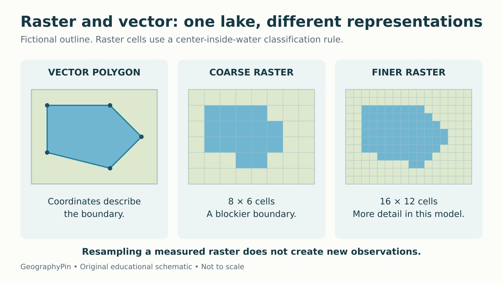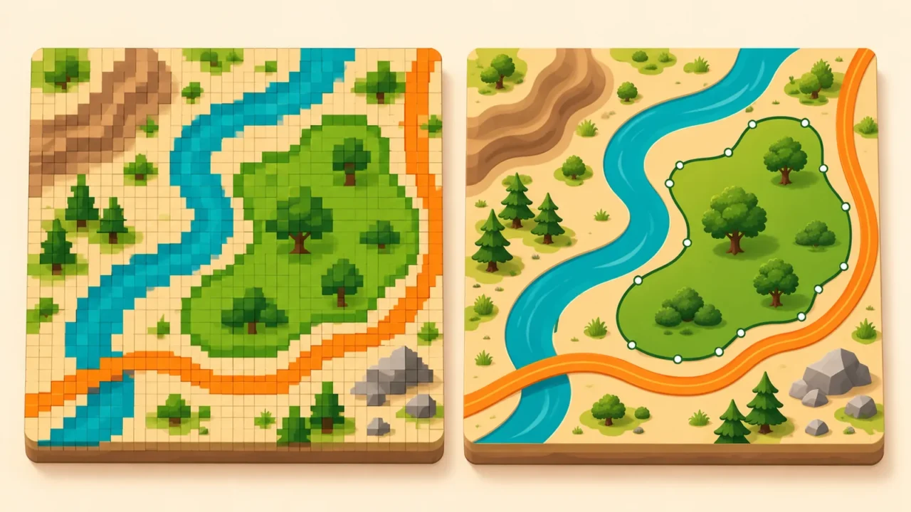
The same lake can appear as a polygon outline or as a set of colored grid cells. Both can be useful geographic data, but they store and simplify the landscape in different ways.
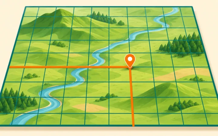
Raster data divide space into rows and columns of cells, each holding a value. Vector data represent features with coordinate-based geometry, commonly points, lines and polygons, linked to descriptive attributes. Raster is often useful for imagery and surfaces; vector is often useful for distinct objects and networks. Neither model is automatically more accurate.
How to use this article: You can read vector geometry, check the cell-size example, or understand conversion limits.
Two Data Models, Not Two Kinds of Reality
A data model determines how geographic information is organized. It does not divide the world permanently into “raster things” and “vector things.” A river might be a line in a national network, a polygon showing its channel width, or water-class cells in a land-cover grid.
The task determines the representation: river connections for routing, channel area for land-cover comparisons, or water characteristics at sampling points require different information.
| Property | Raster | Vector |
|---|---|---|
| Basic structure | Rows and columns of cells | Coordinate-based feature geometry |
| Typical stored value | A measurement, category code or image-band value | Feature attributes attached to geometry |
| Common examples | Elevation grid, land-cover classes, imagery | Entrances, roads, parcel boundaries |
| Main detail control | Cell size and information in the source | Geometry detail and information in the source |
| Typical strength | Cell-by-cell surface operations | Feature and network relationships |
| Important caution | Small cells do not guarantee new detail | Sharp outlines do not guarantee accurate boundaries |
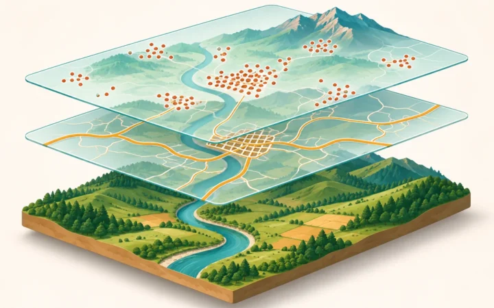
GIS projects often combine both: rainfall cells can be summarized inside watershed polygons, or imagery can provide context for mapped features. Choose the representation for the question.
Vector: Features, Vertices and Attributes
Geometry describes the shape; attributes describe the feature
A point records a position. A line connects positions into a path. A polygon describes an enclosed area, potentially with holes or several parts depending on the dataset. These geometries can carry attributes such as a name, type, date or measured value.
A city shown as a point on a continental map does not occupy zero area in reality. The point is a representation chosen for that scale and purpose. At a more detailed scale, a city boundary may be stored as a polygon. QGIS’s vector-data guide uses this distinction to explain feature choice.
Geometry and connectivity are also different. Two road lines can cross on a screen while representing a bridge and the road beneath it, with no junction between them. A routing network needs the correct connections and travel rules, not merely intersecting strokes.
A displayed line’s width is a symbol choice, not necessarily a measurement of the feature’s real width. Check the legend and dataset description.
Raster: Cells, Bands and Meaning
A raster covers an extent with a regular grid. In a simple one-band elevation raster, each cell contains a height value. In a land-cover raster, it may contain a code for a class such as water or forest. An image may have several bands recording different portions of the electromagnetic spectrum or other quantities.
The numbers need a definition. A cell value of 3 could mean a land-cover class, a measured quantity or something else entirely. Three forest cells are not necessarily three trees, and a value of 3 is not automatically three times as much of a property as a value of 1.
NoData also needs separate treatment. It marks a value as absent or invalid under the dataset’s convention; it is not automatically a measured zero. Counting unknown cells as zero rainfall, for example, would change the meaning of an average. GDAL’s raster data-model documentation describes bands, georeferencing, metadata and NoData values.
A grid must be located geographically as well as drawn. Its coordinate reference and the relationship between cell positions and ground coordinates determine where it belongs. A screenshot with colored squares is not automatically a usable georeferenced raster dataset.
What Changing Cell Size Actually Does
Compare the same area at two resolutions
Imagine a square study area 120 meters on each side, roughly 394 feet. A grid with 30-meter cells, about 98 feet, has 4 columns and 4 rows: 16 cells. Using 10-meter cells, about 33 feet, gives 12 columns and 12 rows: 144 cells.
The finer grid has nine times as many cells because the count increases in both directions. Each 30-meter cell covers 900 square meters; each 10-meter cell covers 100 square meters. Those are horizontal grid areas, not measurements of sloping ground.

If the original observations support fine detail, a smaller cell size can preserve more of it. Simply resampling an existing coarse raster into smaller cells does not recover missing details. Esri’s pixel-size guidance makes that limitation explicit.
The same caution applies to vector data: adding vertices or drawing a smoother curve does not improve an uncertain survey. Resolution describes represented detail; accuracy concerns agreement with the relevant reference or reality. Check both, rather than judging quality by how crisp the display looks.
Conversions Change the Representation
Rasterization and vectorization are not perfect reversals
Rasterization turns vector information into cells according to a chosen rule. For a lake polygon, a method might classify cells by their centers or by how much of each cell the polygon covers. Different rules, cell sizes and grid alignments can produce different edge cells.
Vectorization can trace boundaries between raster classes, producing polygons along cell edges. It cannot automatically recover the exact shoreline that existed before the raster was made. Smoothing those edges introduces another modeling decision.
Resampling is another operation: it estimates or assigns values on a new grid. For category codes, a method that invents intermediate values can create meaningless classes. Esri’s resampling guidance recommends nearest neighbor for categorical data and distinguishes methods used for continuous values.
Averaging the codes for water and forest does not produce a valid halfway land-cover class. By contrast, interpolation may be meaningful for a continuous quantity when the method and data assumptions fit. The meaning of the values matters as much as the file extension.
Choose the Representation for the Job
| Task | Likely useful representation | Check before using it |
|---|---|---|
| Count recorded entrances | Vector points | Unique IDs, completeness and dates |
| Follow connected roads | Vector network | Junctions, direction and access rules |
| Analyze elevation across an area | Elevation raster or another terrain model | Vertical reference, cell size and accuracy |
| Inspect satellite measurements | Raster bands | Band meanings, processing and missing values |
| Summarize values by district | District polygons plus the relevant data | Boundary date and summary method |
Point clouds, meshes and other geographic data models also exist.
Before combining files, check their coordinate reference systems, units, dates, extent, resolution or capture scale, and reuse conditions. For raster calculations, matching cell size alone may not be enough: cell alignment and NoData treatment can affect the result.
Finally, distinguish stored data from display. A vector dataset can be rendered into image tiles, and a raster can be styled with smooth colors. The picture on screen may hide the original structure. GeographyPin’s map-reading guide explains the separate job of interpreting scale and symbols, while the GIS quiz tests the underlying concepts.
What Did We Learn Today?
Raster and vector organize geographic evidence differently, but both simplify the world. Cell values need definitions, feature geometry needs context, and neither small pixels nor smooth outlines guarantee accuracy. The best choice follows the task, preserves the meaning of the observations and records what changed during conversion or analysis.
Sources & Data Notes
The lake diagram and cell-count exercise are original fictional examples. The diagram uses a stated cell-center rule and is not derived from a surveyed shoreline. Metric dimensions are retained for exact grid arithmetic; approximate feet are included for orientation. Software documentation supports general concepts, not a promise that all formats or tools behave identically.