A dark patch on a statistical map may show a high percentage, a high density or another measured value. It does not automatically mean “the most people.” Reading the title and legend is only the start; the denominator and boundaries matter too.
A choropleth map fills geographic areas with colors or shades linked to a numerical value, commonly a rate, percentage or density. The shading summarizes each area rather than locating every observation. To read it correctly, check what is measured, what it is divided by, how the color classes work and which boundaries define the areas.
How to use this article: You can identify the mapped measure, compare counts with shares, interpret the legend, or recognize area-level limits.
Identify the Measure Before Reading the Pattern
A shaded area represents a summary
Choropleth maps commonly use countries, counties, districts or census areas as their units. Each unit receives a shade based on its data value. The map is useful when the geographic pattern itself is part of the question.
The UK Office for National Statistics recommends considering other charts when a map adds little, especially with only a few areas. A bar chart usually makes exact comparisons easier. The small schematic below uses four fictional districts to teach the reading method, not to argue that every four-row dataset needs a map.
Begin by identifying the variable and units: percentage of households, people per square mile, median income or something else. A density has an area denominator, while a percentage describes a share of a specified total. Those measures answer different questions even when both appear as dark and light shading.
Use the Denominator That Matches the Question
More observations can still mean a smaller share
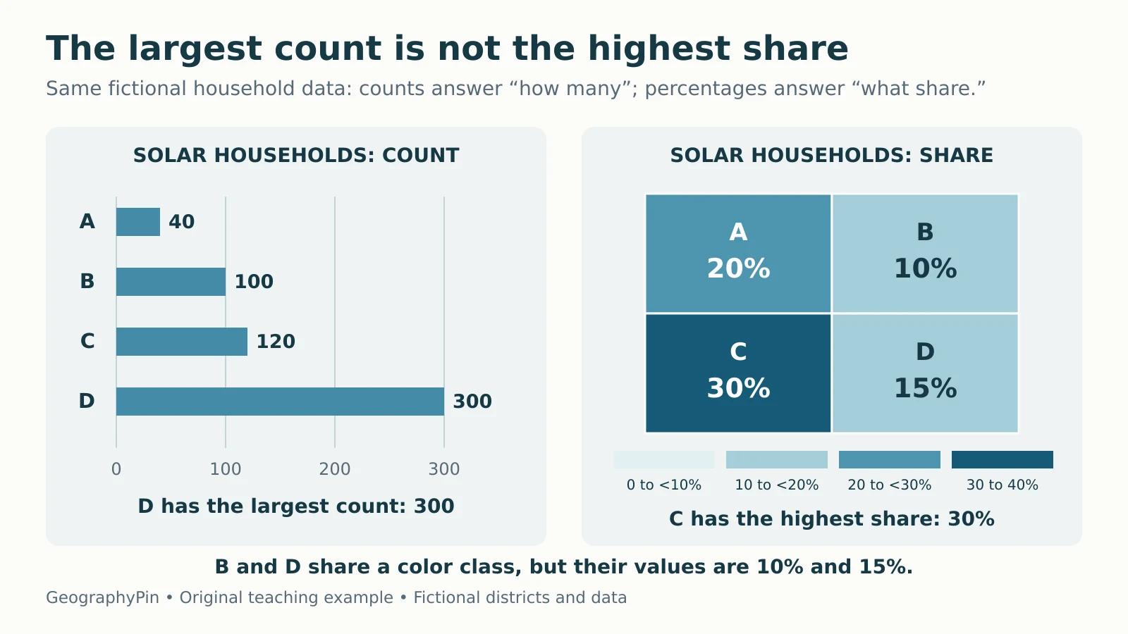
Suppose a fictional survey records households using rooftop solar. To compare the share of households, divide solar households by all households in the same district and multiply by 100.
| District | All households | Solar households | Share with solar |
|---|---|---|---|
| A | 200 | 40 | 20% |
| B | 1,000 | 100 | 10% |
| C | 400 | 120 | 30% |
| D | 2,000 | 300 | 15% |
D has the largest count, 300, but C has the largest share, 120 ÷ 400 × 100 = 30%. D’s share is only 300 ÷ 2,000 × 100 = 15%. Neither number is wrong: one answers “how many,” and the other answers “what proportion.”

Download the example data as CSV. Esri’s normalization guide explains why proportional or graduated symbols are generally better for mapping counts, while shaded areas usually suit derived values.
The denominator must describe the relevant group. Household counts divided by population do not produce the percentage of households. Penn State’s cartography guidance emphasizes matching the measured group to the appropriate total. Dividing by area would instead answer a density question.
Treat a Color Class as a Range, Not an Exact Value
Check which side owns a boundary value
In the example, the four classes are 0% to less than 10%, 10% to less than 20%, 20% to less than 30%, and 30% through 40%. Thus B at 10% and D at 15% share a color. A at exactly 20% belongs to the next class, and C at 30% belongs to the darkest class.
These breaks are explicit teaching choices. A real legend may use other intervals or a continuous scale. Read its endpoints carefully. Two areas with the same shade need not have equal values, and a small difference near a class boundary can produce different shades.
Also identify the palette. A sequential scale usually progresses from lower to higher values. A diverging scale emphasizes values on opposite sides of a meaningful midpoint, such as zero change. Darker can therefore mean a more extreme departure in either direction rather than simply “more.”
A category map assigning different colors to land-cover types is another kind of thematic map; its colors need not have a low-to-high order. The legend tells you which interpretation applies.
Classification Can Change the Visual Message
The same numeric values can look different when grouped differently. ArcGIS documentation describes several common approaches:
| Method | Basic rule | Reading caution |
|---|---|---|
| Equal interval | Divide the numeric range into equal-width bands | Some bands may contain few or no areas |
| Quantile | Aim for similar numbers of areas per class | Similar values may be separated; unlike values may be grouped |
| Natural breaks | Group similar values using the distribution of the dataset | Breaks can change when the underlying dataset changes |
No method is automatically right for every purpose. A fixed meaningful threshold may matter more than making the colors look balanced. With quantiles, equal class counts also do not mean equal populations or equal land areas.
When comparing maps from different years, check that their values, definitions, boundaries and breaks are comparable. Two maps can use identical colors but assign those colors to different ranges. A darker-looking map does not establish growth until you check the scales.
Keep Area-Level Conclusions at the Area Level
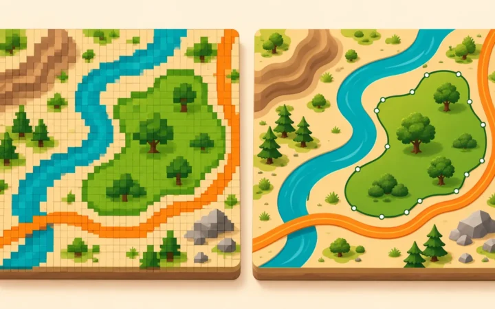
A district color does not locate every household
C’s 30% share does not mean every street has 30% solar households. The households could be concentrated in one neighborhood. Uniform fill is a display choice, not evidence of uniform distribution.
Inferring individual characteristics from an aggregate pattern risks the ecological fallacy. Changing the size or arrangement of the areas can also change aggregate results, a problem known as the modifiable areal unit problem. The UCGIS statistical-mapping chapter explains both limitations.
For example, combining all four fictional districts requires adding the underlying counts: 560 solar households out of 3,600 households gives about 15.6%. The unweighted average of 20%, 10%, 30% and 15% is 18.75%, which answers a different question: the mean of four district percentages. It is not the share of all households combined.
Large regions can also dominate the page visually without containing most of the people. Keep geographic area, population and the mapped statistic separate.
Use a Short Checklist Before Drawing Conclusions
- Measure: What is the variable, date and unit?
- Denominator: Is this a count, rate, percentage, density or other summary?
- Legend: What do the classes, endpoints and palette mean?
- Geography: Which boundaries and level of aggregation are used?
- Data quality: Are missing or suppressed values identified separately from zero, and are estimates accompanied by relevant uncertainty?
- Claim: Does the conclusion describe areas, or does it improperly assume individual locations or circumstances?
Zero and missing are not interchangeable. A district with no recorded value cannot safely be assigned a 0% share, and division by a zero denominator does not produce a valid percentage.
The cartography quiz tests rates and legend ranges, while the GIS quiz explores aggregation and data-quality pitfalls. Use those checks to read the map’s evidence rather than just its strongest color.
What Did We Learn Today?
A choropleth map summarizes a numeric value within geographic areas. Read the variable, denominator and class boundaries before interpreting its pattern. Counts and shares answer different questions, shared colors need not mean equal values, and changing boundaries or classification can alter the picture. Keep conclusions at the scale the data actually support.
Sources & Data Notes
All four districts, household counts, positions and shapes are fictional. Percentages are computed from the supplied CSV, and the combined share is rounded to one decimal place. The illustrative class ranges run from 0% to 40% and cover every example value. No real solar-adoption ranking or geographic trend is implied.