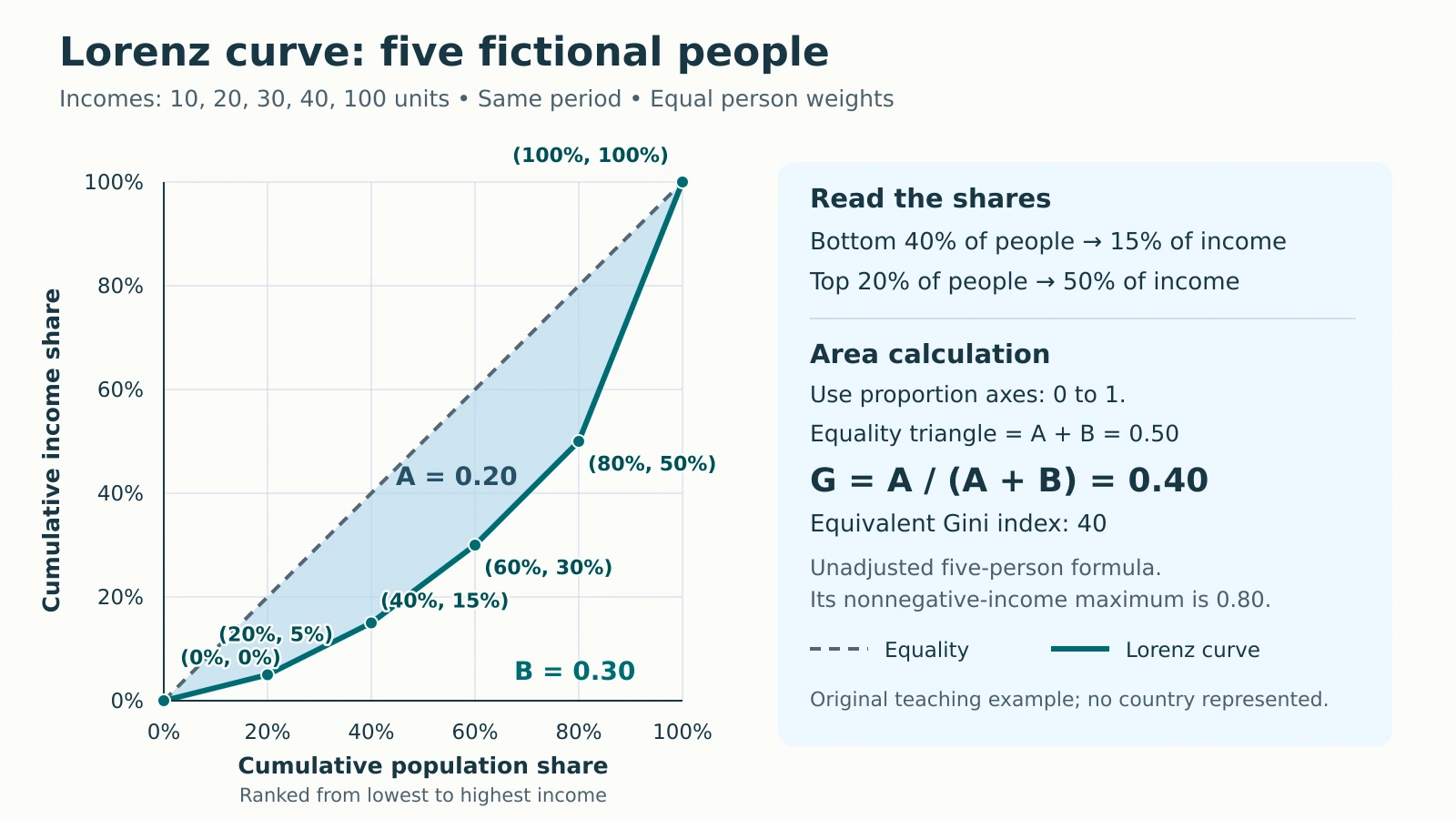
A Lorenz curve shows how income is shared, while a Gini coefficient reduces that distribution to one number. Reading both requires keeping cumulative percentages separate from income amounts and checking how the statistic was calculated.
Read a Lorenz curve by matching a cumulative share of people, ranked from lowest to highest income, to their cumulative share of total income. The equality line gives equal shares to equal population shares. The Gini coefficient summarizes the gap between the curve and that line, using a stated calculation convention.
How to use this article: You can read the example’s shares, calculate the shaded gap, or check grouped data.
Read the Axes in Income Order
Begin with the population, income definition and time period. Then sort the records from lowest to highest income. The Office for National Statistics describes this cumulative ranking approach.
The horizontal axis adds people; the vertical axis adds their income. Both show shares of their respective totals, from 0% to 100%. Cumulative means including everyone up to that rank, not just the last person added.
On the equality line, the bottom 40% receive 40% of income. With unequal nonnegative incomes and a positive total, the Lorenz curve lies below that line somewhere. Neither axis locates people geographically, so spatial analysis in human geography needs additional location data.
Build the Curve from Five People
Our entire fictional population consists of five equally weighted people receiving 10, 20, 30, 40 and 100 units over the same period. These are arbitrary income units, not country statistics. Total income is 200 units, and mean income is 200 ÷ 5 = 40.
| Person by rank | Income, units | Cumulative income, units | Population share | Income share |
|---|---|---|---|---|
| Start | Not applicable | 0 | 0% | 0% |
| 1 | 10 | 10 | 20% | 5% |
| 2 | 20 | 30 | 40% | 15% |
| 3 | 30 | 60 | 60% | 30% |
| 4 | 40 | 100 | 80% | 50% |
| 5 | 100 | 200 | 100% | 100% |
The last two columns are cumulative. Each person adds 20 percentage points of population. Divide cumulative income by 200: after person 2, 30 ÷ 200 = 15%. Plot those two columns, including the origin, and join adjacent points with straight segments. Do not smooth the line: the segment slopes represent the successive individual incomes. The final point must reach 100% on both axes because everyone and all income have been counted.

Read the bottom share, then find the top share
At 40% along the horizontal axis, the curve reaches 15% vertically: the lowest-income two people receive 15% of total income. At 80%, cumulative income is 50%, so the remaining top 20% receive 100% − 50% = 50%. Reading the 80% point directly as the top group’s share would reverse its meaning.
Calculate the Gini from the Area
Add five trapezoids beneath the curve
Convert percentages to proportions before calculating areas: 20% becomes 0.20. Each segment spans 0.20 horizontally. Its trapezoid area equals that width multiplied by the average of its two endpoint heights.
The first area is 0.20 × (0 + 0.05) ÷ 2 = 0.005. The five areas are 0.005 + 0.020 + 0.045 + 0.080 + 0.150 = 0.300. Call their sum B.
The triangle under equality has area ½ × 1 × 1 = 0.500. Its gap above our curve is 0.500 − 0.300 = 0.200. Therefore G = 0.200 ÷ 0.500 = 1 − 2B = 0.400. A coefficient of 0.40 is the same result as a Gini index of 40 on the 0–100 scale.
As an independent check, sum absolute income differences over all 25 ordered pairs, including both directions and zero self-differences. Their sum is 800. Dividing by twice the number of people times total income gives 800 ÷ (2 × 5 × 200) = 0.40.
Five-person convention: this unadjusted formula has a maximum of 1 − 1/5 = 0.8 for nonnegative incomes, attained when one person receives everything. Statistics Canada gives this finite-population limit. Multiplying by n/(n−1), where n is the number of people, would instead give 0.50 here. That changes the convention; we do not apply it. The usual theoretical upper limit of 1 should not be mistaken for an attainable value of this five-person polygon.
Separate Income Level from Distribution
Give each person 40 units instead. The total remains 200 and the mean remains 40, but every cumulative income share now equals its population share. The curve follows equality, so G = 0.
Alternatively, double every original income to 20, 40, 60, 80 and 200. The total becomes 400 and the mean 80. Every income share stays unchanged, so the curve and G = 0.40 remain unchanged.
These comparisons separate relative distribution from income level. These arithmetic comparisons say nothing about prices or purchasing power. GDP per person and wealth describe other quantities.
Check Real-World Definitions and Grouping
Before comparing published figures, check:
- Variable: income or consumption, and before or after taxes and transfers. The OECD indicator specifically uses household disposable income.
- Population: people or households, survey weights, coverage, and household-size adjustments. Equivalization adjusts for household size and composition.
- Period and method: survey year, calculation convention, and treatment of zero or negative incomes.
Quintile shares leave information between the points
Our five records are individuals. Five quintiles in a larger population are different: each group contains one-fifth of the people. Joining only their cumulative shares with straight lines treats incomes within each group as equal. Without within-group equality, that area-based Gini is a lower-bound approximation, not the exact all-person result. Jordá, Sarabia and Jäntti’s grouped-data study explains the missing within-group variation.
Negative incomes also require care. The Australian Bureau of Statistics notes that business losses can produce Ginis above 1. Negative amounts can take part of a Lorenz curve below zero; providers may handle them differently. The familiar 0–1 range is not universal for signed data. An all-zero total cannot supply income shares through this formula.
Write Only What the Evidence Supports
A defensible reading is: “In this five-person example, the bottom 40% receive 15% of income, the top 20% receive 50%, and the unadjusted Gini is 0.40.” That 40 is neither the richest person’s share nor the percentage of people who are poor. A poverty rate requires a defined threshold.
A change from 0.40 to 0.42 would be two Gini index points, not a 2% relative increase. The curve does not explain causes, map residences or track individual mobility. Different curves can share one Gini. If two curves cross, neither is closer to equality at every population share. Regional Ginis also cannot simply be averaged into a national Gini.
What Did We Learn Today?
Sort incomes, calculate cumulative shares and read the two axes together. Our five-person curve gives bottom-40% and top-20% shares of 15% and 50%, with an unadjusted Gini of 0.40. Doubling incomes preserves that relative distribution. Before comparing real figures, check definitions, population, grouping and calculation conventions.
Sources & Data Notes
All five incomes and the original diagram are fictional. Calculations use equally weighted individual records, straight segments and the unadjusted all-pairs Gini. Displayed shares and areas are exact for this example; no survey or country ranking is represented.